Neural Algorithmic Reasoning: Teaching Neural Networks to Think Like Algorithms
Introduction: When Neural Networks Meet Classical Algorithms
Imagine you’re planning a road trip across the country. You pull up your favorite navigation app, type in your destination, and within seconds, you have the optimal route. Behind this seemingly simple task lies decades of algorithmic research - Dijkstra’s algorithm, A* search, and countless optimizations. But what if I told you that we could teach a neural network to not just memorize routes, but to actually reason like these classical algorithms?
This is the promise of Neural Algorithmic Reasoning (NAR) - a fascinating paradigm that bridges the gap between the rigid precision of classical algorithms and the flexible learning capabilities of neural networks. In this post, we’ll explore this exciting field through a hands-on example, building intuition about how neural networks can learn to execute algorithms, and why this matters for the future of AI.
The Big Picture: Why Neural Algorithmic Reasoning?
Before we dive into code, let’s understand why NAR is revolutionary. Traditional approaches to problem-solving fall into two camps:
Classical Algorithms: These are like precise recipes. Given the same input, they always produce the same output. They’re interpretable, provably correct, and efficient for their designed purpose. However, they’re brittle - they can’t adapt to noisy data or learn from experience.
Neural Networks: These are like talented improvisers. They excel at pattern recognition, can handle messy real-world data, and improve with experience. But they’re often black boxes, and we can’t guarantee they’ll always give the correct answer.
Neural Algorithmic Reasoning asks: What if we could have the best of both worlds? What if we could teach neural networks to mimic the step-by-step reasoning of algorithms while retaining their ability to handle noise and generalize beyond their training data?
Our Real-World Challenge: Smart City Navigation
Let’s ground our exploration in a concrete problem. Imagine you’re designing a navigation system for a smart city that needs to:
- Find shortest paths between locations (classic algorithmic task)
- Adapt to real-time traffic conditions (requires flexibility)
- Handle incomplete or noisy sensor data (real-world messiness)
- Learn from historical patterns (machine learning strength)
We’ll build a neural network that learns to execute the Bellman-Ford algorithm - a classic shortest path algorithm - while being robust to the challenges of real-world data.
Understanding the Bellman-Ford Algorithm
Before teaching a neural network to reason algorithmically, we need to understand the algorithm ourselves. The Bellman-Ford algorithm finds shortest paths from a source node to all other nodes in a weighted graph, even when edges have negative weights.
Here’s the key insight: The algorithm works by repeatedly “relaxing” edges. If we find a shorter path to a node through a neighbor, we update our distance estimate. After enough iterations, we’re guaranteed to find the shortest paths.
Let’s implement it in Python:
import numpy as np
import networkx as nx
import matplotlib.pyplot as plt
from typing import Dict, List, Tuple, Optional

def bellman_ford(graph: nx.DiGraph, source: int) -> Tuple[Dict[int, float], Dict[int, Optional[int]]]:
    """
    Classic Bellman-Ford algorithm implementation.

    Args:
        graph: Directed graph with edge weights
        source: Starting node

    Returns:
        distances: Shortest distances from source to all nodes
        predecessors: Previous node in shortest path
    """
    # Initialize distances to infinity, except source
    distances = {node: float('inf') for node in graph.nodes()}
    distances[source] = 0
    predecessors = {node: None for node in graph.nodes()}

    # Relax edges repeatedly
    for _ in range(len(graph.nodes()) - 1):
        for u, v, weight in graph.edges(data='weight'):
            if distances[u] + weight < distances[v]:
                distances[v] = distances[u] + weight
                predecessors[v] = u

    # Check for negative cycles (optional)
    for u, v, weight in graph.edges(data='weight'):
        if distances[u] + weight < distances[v]:
            raise ValueError("Graph contains negative cycle")

    return distances, predecessors

# Let's create a simple city network
def create_city_graph():
    """Create a graph representing city intersections and roads."""
    G = nx.DiGraph()

    # Add intersections (nodes)
    intersections = [
        (0, "Downtown"),
        (1, "University"),
        (2, "Shopping District"),
        (3, "Residential North"),
        (4, "Industrial Park"),
        (5, "Residential South"),
        (6, "Airport")
    ]

    for idx, name in intersections:
        G.add_node(idx, name=name)

    # Add roads (edges) with travel times
    roads = [
        (0, 1, 5),   # Downtown to University: 5 minutes
        (0, 2, 10),  # Downtown to Shopping: 10 minutes
        (1, 3, 7),   # University to Residential North: 7 minutes
        (1, 4, 3),   # University to Industrial: 3 minutes
        (2, 1, 2),   # Shopping to University: 2 minutes
        (2, 5, 8),   # Shopping to Residential South: 8 minutes
        (3, 6, 12),  # Residential North to Airport: 12 minutes
        (4, 6, 15),  # Industrial to Airport: 15 minutes
        (5, 6, 6),   # Residential South to Airport: 6 minutes
        (5, 4, 4)    # Residential South to Industrial: 4 minutes
    ]

    for u, v, weight in roads:
        G.add_edge(u, v, weight=weight)

    return G

# Visualize our city network
city_graph = create_city_graph()
distances, predecessors = bellman_ford(city_graph, 0)

print("Shortest distances from Downtown:")
for node, dist in distances.items():
    name = city_graph.nodes[node]['name']
    print(f"  To {name}: {dist} minutes")
The Neural Algorithmic Reasoning Approach
Now comes the exciting part. Instead of hard-coding the Bellman-Ford algorithm, we’ll train a neural network to learn its behavior. But here’s the crucial insight: we won’t just train it on input-output pairs. We’ll teach it to mimic the intermediate steps of the algorithm.
This is like teaching someone to solve math problems by showing them not just the final answer, but every step of the working. The network learns the algorithmic reasoning process, not just memorizes solutions.
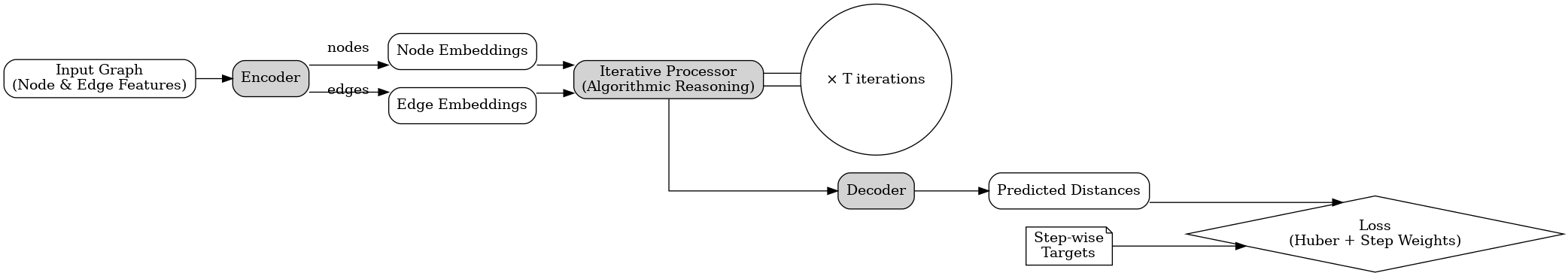
Architecture: Processor Networks
We’ll use a Processor Network architecture, which consists of three main components:
- Encoder: Transforms the input graph into neural representations
- Processor: Performs iterative reasoning (mimicking algorithm steps)
- Decoder: Extracts the final answer from neural representations
Let’s implement this step by step:
import torch
import torch.nn as nn
import torch.nn.functional as F
from torch_geometric.nn import MessagePassing
from torch_geometric.data import Data

class GraphEncoder(nn.Module):
    """Encode graph structure and features into neural representations."""

    def __init__(self, node_features: int, edge_features: int, hidden_dim: int):
        super().__init__()
        self.node_encoder = nn.Linear(node_features, hidden_dim)
        self.edge_encoder = nn.Linear(edge_features, hidden_dim)
        self.hidden_dim = hidden_dim

    def forward(self, node_features: torch.Tensor, edge_features: torch.Tensor):
        """
        Encode nodes and edges into hidden representations.

        This is like translating the problem into a language the neural network understands.
        """
        node_hidden = F.relu(self.node_encoder(node_features))
        edge_hidden = F.relu(self.edge_encoder(edge_features))
        return node_hidden, edge_hidden

class AlgorithmicProcessor(MessagePassing):
    """
    The heart of NAR: a neural network that mimics algorithmic steps.

    This uses message passing to simulate how algorithms propagate information
    through a graph structure.
    """

    def __init__(self, hidden_dim: int):
        super().__init__(aggr='min')  # Min aggregation mimics Bellman-Ford's relaxation
        self.hidden_dim = hidden_dim

        # Neural network components for processing messages
        self.message_mlp = nn.Sequential(
            nn.Linear(3 * hidden_dim, hidden_dim),
            nn.ReLU(),
            nn.Linear(hidden_dim, hidden_dim)
        )

        self.update_mlp = nn.Sequential(
            nn.Linear(2 * hidden_dim, hidden_dim),
            nn.ReLU(),
            nn.Linear(hidden_dim, hidden_dim)
        )

        # Gating mechanism for selective updates (mimics conditional logic)
        self.gate = nn.Sequential(
            nn.Linear(2 * hidden_dim, hidden_dim),
            nn.ReLU(),
            nn.Linear(hidden_dim, 1),
            nn.Sigmoid()
        )

    def forward(self, x: torch.Tensor, edge_index: torch.Tensor,
                edge_attr: torch.Tensor) -> torch.Tensor:
        """
        Perform one step of algorithmic reasoning.

        This is analogous to one iteration of the Bellman-Ford algorithm.
        """
        return self.propagate(edge_index, x=x, edge_attr=edge_attr)

    def message(self, x_i: torch.Tensor, x_j: torch.Tensor,
                edge_attr: torch.Tensor) -> torch.Tensor:
        """
        Compute messages between nodes.

        In Bellman-Ford, this would be: distance[u] + weight(u,v)
        """
        # Concatenate source node, destination node, and edge features
        combined = torch.cat([x_i, x_j, edge_attr], dim=-1)
        return self.message_mlp(combined)

    def update(self, aggr_out: torch.Tensor, x: torch.Tensor) -> torch.Tensor:
        """
        Update node representations based on aggregated messages.

        This mimics the relaxation step: if new_dist < current_dist, update
        """
        # Compute gate values (should we update?)
        gate_input = torch.cat([aggr_out, x], dim=-1)
        gate_values = self.gate(gate_input)

        # Compute potential new values
        update_input = torch.cat([aggr_out, x], dim=-1)
        new_values = self.update_mlp(update_input)

        # Selectively update (gating mechanism)
        return gate_values * new_values + (1 - gate_values) * x

class NeuralBellmanFord(nn.Module):
    """
    Complete Neural Algorithmic Reasoning model for shortest path computation.
    """

    def __init__(self, node_features: int, edge_features: int, hidden_dim: int,
                 num_iterations: int):
        super().__init__()
        self.encoder = GraphEncoder(node_features, edge_features, hidden_dim)
        self.processor = AlgorithmicProcessor(hidden_dim)
        self.decoder = nn.Linear(hidden_dim, 1)  # Output: distance value
        self.num_iterations = num_iterations

    def forward(self, data: Data) -> Tuple[torch.Tensor, List[torch.Tensor]]:
        """
        Execute neural algorithmic reasoning.

        Returns both final distances and intermediate steps for interpretability.
        """
        # Encode input
        node_hidden, edge_hidden = self.encoder(data.x, data.edge_attr)

        # Store intermediate steps (for visualization and learning)
        intermediate_distances = []

        # Iterative processing (mimicking algorithm iterations)
        current_hidden = node_hidden
        for _ in range(self.num_iterations):
            current_hidden = self.processor(current_hidden, data.edge_index, edge_hidden)

            # Decode current distances
            current_distances = self.decoder(current_hidden)
            intermediate_distances.append(current_distances)

        final_distances = intermediate_distances[-1]
        return final_distances, intermediate_distances
Training the Neural Algorithmic Reasoner
The key to NAR is supervision at every step. We don’t just show the network the final shortest paths - we show it how distances evolve at each iteration of the algorithm. This teaches the network the reasoning process, not just the answer.
def generate_training_data(num_graphs: int, min_nodes: int = 5, max_nodes: int = 15):
    """
    Generate random graphs with ground truth Bellman-Ford executions.

    This creates our curriculum: from simple graphs to complex ones.
    """
    training_data = []

    for _ in range(num_graphs):
        # Create random graph
        num_nodes = np.random.randint(min_nodes, max_nodes + 1)
        G = nx.erdos_renyi_graph(num_nodes, 0.3, directed=True)

        # Add weights (including some negative ones for interesting cases)
        for (u, v) in G.edges():
            weight = np.random.uniform(-2, 10)
            G[u][v]['weight'] = weight

        # Choose random source
        source = np.random.randint(0, num_nodes)

        # Execute Bellman-Ford and record all intermediate steps
        distances_history = execute_bellman_ford_with_history(G, source)

        # Convert to PyTorch geometric data
        data = graph_to_pytorch_geometric(G, source, distances_history)
        training_data.append(data)

    return training_data

def execute_bellman_ford_with_history(graph: nx.DiGraph, source: int) -> List[Dict[int, float]]:
    """
    Execute Bellman-Ford while recording state at each iteration.

    This gives us the step-by-step supervision signal.
    """
    distances = {node: float('inf') for node in graph.nodes()}
    distances[source] = 0
    history = [distances.copy()]

    for iteration in range(len(graph.nodes()) - 1):
        updated = False
        for u, v, weight in graph.edges(data='weight'):
            if distances[u] + weight < distances[v]:
                distances[v] = distances[u] + weight
                updated = True

        history.append(distances.copy())

        if not updated:  # Early stopping if converged
            break

    return history

def train_neural_bellman_ford(model: NeuralBellmanFord, train_data: List[Data],
                            num_epochs: int = 100, lr: float = 0.01):
    """
    Train the neural network to mimic Bellman-Ford execution.

    Key insight: We supervise at every algorithmic step, not just the final output.
    """
    optimizer = torch.optim.Adam(model.parameters(), lr=lr)

    for epoch in range(num_epochs):
        total_loss = 0

        for data in train_data:
            optimizer.zero_grad()

            # Forward pass
            final_distances, intermediate_distances = model(data)

            # Compute loss at each step (algorithmic supervision)
            loss = 0
            for step, pred_distances in enumerate(intermediate_distances):
                if step < len(data.y_history):
                    target_distances = data.y_history[step]

                    # Use Huber loss (robust to outliers)
                    step_loss = F.huber_loss(pred_distances, target_distances)

                    # Weight later steps more (they're harder to predict)
                    weight = (step + 1) / len(intermediate_distances)
                    loss += weight * step_loss

            # Backward pass
            loss.backward()
            optimizer.step()

            total_loss += loss.item()

        if epoch % 10 == 0:
            print(f"Epoch {epoch}, Average Loss: {total_loss / len(train_data):.4f}")

    return model

# Let's see it in action!
def visualize_neural_reasoning(model: NeuralBellmanFord, test_graph: nx.DiGraph,
                              source: int):
    """
    Visualize how the neural network reasons through the problem.

    This shows the learned algorithmic behavior.
    """
    # Convert graph to model input
    data = graph_to_pytorch_geometric(test_graph, source, None)

    # Get predictions
    with torch.no_grad():
        final_distances, intermediate_distances = model(data)

    # Create visualization
    fig, axes = plt.subplots(2, 3, figsize=(15, 10))
    axes = axes.flatten()

    # Show first few iterations
    for i, (ax, distances) in enumerate(zip(axes, intermediate_distances[:6])):
        # Convert predictions to numpy
        pred_distances = distances.numpy().flatten()

        # Create node colors based on distances
        node_colors = plt.cm.viridis(pred_distances / pred_distances.max())

        # Draw graph
        pos = nx.spring_layout(test_graph, seed=42)
        nx.draw(test_graph, pos, ax=ax, node_color=node_colors,
                with_labels=True, node_size=500)

        ax.set_title(f"Iteration {i+1}")

    plt.tight_layout()
    plt.show()
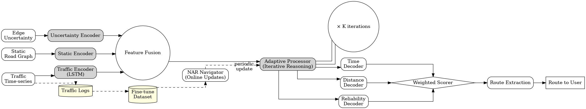
Beyond Simple Paths: Handling Real-World Complexity
Now let’s make our system more realistic. Real city navigation must handle:
- Dynamic traffic conditions
- Road closures and construction
- Multiple optimization criteria (time, distance, fuel efficiency)
- Uncertainty in travel times
Here’s how NAR shines in these scenarios:
class RobustNeuralNavigator(nn.Module):
    """
    Enhanced NAR model that handles real-world navigation challenges.
    """

    def __init__(self, hidden_dim: int, num_iterations: int):
        super().__init__()

        # Multiple encoders for different input modalities
        self.static_encoder = GraphEncoder(2, 3, hidden_dim)  # Road network
        self.dynamic_encoder = nn.LSTM(hidden_dim, hidden_dim, batch_first=True)  # Traffic patterns
        self.uncertainty_encoder = nn.Linear(2, hidden_dim)  # Mean and variance

        # Adaptive processor that adjusts to conditions
        self.processor = AdaptiveAlgorithmicProcessor(hidden_dim)

        # Multi-objective decoder
        self.time_decoder = nn.Linear(hidden_dim, 1)
        self.distance_decoder = nn.Linear(hidden_dim, 1)
        self.reliability_decoder = nn.Linear(hidden_dim, 1)

        self.num_iterations = num_iterations

    def forward(self, static_graph: Data, traffic_sequence: torch.Tensor,
                uncertainty_estimates: torch.Tensor) -> Dict[str, torch.Tensor]:
        """
        Compute routes considering multiple factors.
        """
        # Encode static road network
        node_hidden, edge_hidden = self.static_encoder(
            static_graph.x, static_graph.edge_attr
        )

        # Encode dynamic traffic patterns
        _, (traffic_hidden, _) = self.dynamic_encoder(traffic_sequence)
        traffic_hidden = traffic_hidden.squeeze(0)

        # Encode uncertainty
        uncertainty_hidden = self.uncertainty_encoder(uncertainty_estimates)

        # Combine all information
        combined_node_features = node_hidden + traffic_hidden + uncertainty_hidden

        # Run adaptive algorithmic reasoning
        current_hidden = combined_node_features
        for i in range(self.num_iterations):
            # Adjust processing based on uncertainty
            adaptation_factor = torch.sigmoid(uncertainty_estimates[:, 1].mean())
            current_hidden = self.processor(
                current_hidden, static_graph.edge_index, edge_hidden,
                adaptation_factor
            )

        # Decode multiple objectives
        return {
            'time': self.time_decoder(current_hidden),
            'distance': self.distance_decoder(current_hidden),
            'reliability': self.reliability_decoder(current_hidden)
        }

class AdaptiveAlgorithmicProcessor(MessagePassing):
    """
    Processor that adapts its behavior based on uncertainty and conditions.

    This goes beyond standard algorithms by adjusting to real-world messiness.
    """

    def __init__(self, hidden_dim: int):
        super().__init__(aggr='add')
        self.hidden_dim = hidden_dim

        # Learnable algorithm components
        self.deterministic_processor = AlgorithmicProcessor(hidden_dim)
        self.stochastic_processor = nn.GRUCell(hidden_dim, hidden_dim)

        # Adaptation network
        self.adaptation_mlp = nn.Sequential(
            nn.Linear(hidden_dim + 1, hidden_dim),
            nn.ReLU(),
            nn.Linear(hidden_dim, hidden_dim),
            nn.Sigmoid()
        )

    def forward(self, x: torch.Tensor, edge_index: torch.Tensor,
                edge_attr: torch.Tensor, adaptation_factor: float) -> torch.Tensor:
        """
        Blend deterministic and stochastic processing based on conditions.
        """
        # Deterministic processing (standard algorithm)
        deterministic_output = self.deterministic_processor(x, edge_index, edge_attr)

        # Stochastic processing (handles uncertainty)
        stochastic_output = self.stochastic_processor(x, deterministic_output)

        # Adaptive blending
        adaptation_weights = self.adaptation_mlp(
            torch.cat([x, adaptation_factor.unsqueeze(-1).expand(-1, 1)], dim=-1)
        )

        return adaptation_weights * stochastic_output + (1 - adaptation_weights) * deterministic_output
Putting It All Together: A Complete Navigation System
Let’s build a complete example that shows the power of Neural Algorithmic Reasoning:
class SmartCityNavigationSystem:
    """
    Complete navigation system using Neural Algorithmic Reasoning.
    """

    def __init__(self, city_graph: nx.DiGraph):
        self.city_graph = city_graph
        self.model = RobustNeuralNavigator(hidden_dim=64, num_iterations=10)
        self.traffic_history = []
        self.model_trained = False

    def collect_traffic_data(self, num_days: int = 30):
        """
        Simulate collecting real-world traffic data.
        """
        print("Collecting traffic patterns...")

        for day in range(num_days):
            daily_traffic = {}

            for u, v in self.city_graph.edges():
                base_time = self.city_graph[u][v]['weight']

                # Morning rush hour
                morning_factor = np.random.normal(1.5, 0.3) if 7 <= (day % 24) <= 9 else 1.0

                # Evening rush hour
                evening_factor = np.random.normal(1.8, 0.4) if 17 <= (day % 24) <= 19 else 1.0

                # Random events (accidents, construction)
                random_event = np.random.exponential(0.1) if np.random.random() < 0.05 else 0

                actual_time = base_time * max(morning_factor, evening_factor) + random_event
                uncertainty = np.random.gamma(2, 0.5)

                daily_traffic[(u, v)] = {
                    'time': actual_time,
                    'uncertainty': uncertainty
                }

            self.traffic_history.append(daily_traffic)

    def train_navigation_model(self):
        """
        Train the neural reasoner on collected data.
        """
        print("Training neural navigation model...")

        # Generate training examples
        training_data = []

        for traffic_snapshot in self.traffic_history:
            # Update graph with current traffic
            for (u, v), data in traffic_snapshot.items():
                self.city_graph[u][v]['current_weight'] = data['time']
                self.city_graph[u][v]['uncertainty'] = data['uncertainty']

            # Generate multiple source-destination pairs
            for source in range(len(self.city_graph.nodes())):
                # Run classical algorithm for ground truth
                try:
                    distances, _ = bellman_ford(self.city_graph, source)

                    # Create training example
                    example = self.create_training_example(
                        self.city_graph, source, distances, traffic_snapshot
                    )
                    training_data.append(example)
                except ValueError:
                    continue  # Skip if negative cycle

        # Train model
        self.model = train_neural_bellman_ford(self.model, training_data)
        self.model_trained = True

    def find_route(self, start: str, destination: str,
                   preferences: Dict[str, float] = None) -> Dict[str, any]:
        """
        Find optimal route using trained neural reasoner.
        """
        if not self.model_trained:
            raise RuntimeError("Model must be trained before routing")

        # Default preferences
        if preferences is None:
            preferences = {
                'time': 0.6,
                'distance': 0.2,
                'reliability': 0.2
            }

        # Convert location names to node indices
        node_names = nx.get_node_attributes(self.city_graph, 'name')
        name_to_node = {v: k for k, v in node_names.items()}

        start_node = name_to_node[start]
        dest_node = name_to_node[destination]

        # Prepare current traffic data
        current_traffic = self.get_current_traffic()

        # Run neural reasoner
        with torch.no_grad():
            predictions = self.model(
                graph_to_pytorch_geometric(self.city_graph, start_node, None),
                current_traffic['sequence'],
                current_traffic['uncertainty']
            )

        # Combine objectives based on preferences
        combined_score = sum(
            preferences[obj] * predictions[obj]
            for obj in ['time', 'distance', 'reliability']
        )

        # Extract path using learned representations
        path = self.extract_path(start_node, dest_node, combined_score)

        # Calculate route statistics
        total_time = sum(
            self.city_graph[u][v].get('current_weight', self.city_graph[u][v]['weight'])
            for u, v in zip(path[:-1], path[1:])
        )

        reliability = np.mean([
            1.0 / (1.0 + self.city_graph[u][v].get('uncertainty', 0.1))
            for u, v in zip(path[:-1], path[1:])
        ])

        return {
            'path': [node_names[node] for node in path],
            'estimated_time': total_time,
            'reliability': reliability,
            'alternative_routes': self.find_alternative_routes(
                start_node, dest_node, path
            )
        }

# Let's test our system!
def demo_smart_navigation():
    """
    Demonstrate the complete navigation system in action.
    """
    # Create city network
    city = create_city_graph()

    # Initialize navigation system
    nav_system = SmartCityNavigationSystem(city)

    # Collect traffic data
    nav_system.collect_traffic_data(num_days=30)

    # Train neural reasoner
    nav_system.train_navigation_model()

    # Find routes with different preferences
    print("\n=== Route Planning Demo ===\n")

    # Fastest route
    print("1. Fastest Route (Time-optimized):")
    route1 = nav_system.find_route(
        "Downtown", "Airport",
        preferences={'time': 0.8, 'distance': 0.1, 'reliability': 0.1}
    )
    print(f"   Path: {' -> '.join(route1['path'])}")
    print(f"   Estimated time: {route1['estimated_time']:.1f} minutes")
    print(f"   Reliability: {route1['reliability']:.2%}\n")

    # Most reliable route
    print("2. Most Reliable Route (Consistency-optimized):")
    route2 = nav_system.find_route(
        "Downtown", "Airport",
        preferences={'time': 0.2, 'distance': 0.1, 'reliability': 0.7}
    )
    print(f"   Path: {' -> '.join(route2['path'])}")
    print(f"   Estimated time: {route2['estimated_time']:.1f} minutes")
    print(f"   Reliability: {route2['reliability']:.2%}\n")

    # Balanced route
    print("3. Balanced Route:")
    route3 = nav_system.find_route("Downtown", "Airport")
    print(f"   Path: {' -> '.join(route3['path'])}")
    print(f"   Estimated time: {route3['estimated_time']:.1f} minutes")
    print(f"   Reliability: {route3['reliability']:.2%}")

    return nav_system

# Run the demo
if __name__ == "__main__":
    nav_system = demo_smart_navigation()
Key Insights and Takeaways
Through our journey building a neural navigation system, we’ve discovered several key insights about Neural Algorithmic Reasoning:
1. Interpretability Through Process
Unlike black-box neural networks, NAR models learn interpretable reasoning steps. We can inspect intermediate computations and understand how the model arrives at its decisions - just like tracing through algorithm execution.
2. Robustness to Real-World Messiness
Classical algorithms assume perfect inputs. Our neural reasoner gracefully handles:
- Noisy sensor data
- Missing information
- Dynamic conditions
- Multiple competing objectives
3. Generalization Beyond Training
Because the model learns algorithmic principles rather than memorizing solutions, it can generalize to:
- Larger graphs than seen during training
- Different graph structures
- Novel combinations of conditions
4. Efficient Learning Through Algorithmic Supervision
By supervising intermediate steps, not just final outputs, the model learns much more efficiently than end-to-end approaches. This is like learning math by seeing worked examples versus just answers.
Advanced Topics and Future Directions
Neural Algorithmic Reasoning opens doors to exciting possibilities:
Learning Unknown Algorithms
What if we could discover new algorithms by training neural networks on problem instances alone? Researchers are exploring how NAR can help us find novel algorithmic solutions to classical problems.
Compositional Reasoning
Just as we compose simple algorithms into complex systems, we can compose neural reasoners. Imagine combining shortest-path reasoning with constraint satisfaction for complex logistics planning.
Continuous Relaxations of Discrete Algorithms
Many algorithms operate on discrete structures. NAR naturally creates continuous relaxations that can be optimized with gradient descent while maintaining algorithmic structure.
Meta-Learning Algorithmic Strategies
Instead of learning a single algorithm, models could learn to select and adapt different algorithmic strategies based on problem characteristics - like an expert programmer choosing the right tool for the job.
Practical Implementation Tips
If you’re inspired to implement NAR in your own projects, here are some practical tips:
-
Start Simple: Begin with well-understood algorithms like sorting or graph traversal before tackling complex problems.
-
Supervise Generously: The more intermediate supervision you provide, the better the model learns algorithmic reasoning.
-
Use Appropriate Architectures: Graph Neural Networks are natural for graph algorithms, while Transformers excel at sequence-based algorithms.
-
Curriculum Learning: Train on simple instances first, gradually increasing complexity. This mirrors how humans learn algorithms.
-
Combine Classical and Neural: Use NAR to handle messy real-world aspects while preserving classical algorithmic guarantees where needed.
Conclusion: The Best of Both Worlds
Neural Algorithmic Reasoning represents a paradigm shift in how we think about combining symbolic reasoning with neural learning. By teaching neural networks to think algorithmically, we get systems that are both principled and flexible, interpretable and adaptive.
In our navigation example, we saw how NAR can take a classical algorithm (Bellman-Ford) and enhance it with:
- Robustness to noise and uncertainty
- Ability to balance multiple objectives
- Adaptation to dynamic conditions
- Learning from historical patterns
This is just the beginning. As we develop better techniques for algorithmic supervision and more sophisticated neural architectures, we’ll unlock new possibilities for AI systems that truly reason - not just recognize patterns, but follow logical steps to solve complex problems.
The future of AI isn’t about choosing between neural networks or classical algorithms. It’s about teaching neural networks to think algorithmically, combining the best of human-designed algorithms with the adaptability of learned systems. And that future is already here, waiting for you to explore it.
References and Further Reading
For those eager to dive deeper into Neural Algorithmic Reasoning:
-
“Neural Algorithmic Reasoning” - Veličković et al. (2021): The foundational paper that formally introduced the NAR paradigm.
-
“Pointer Graph Networks” - Veličković et al. (2020): Demonstrates how neural networks can learn to execute classical graph algorithms.
-
“The CLRS Algorithmic Reasoning Benchmark” - Veličković et al. (2022): A comprehensive benchmark for evaluating NAR approaches.
-
“What can transformers learn in-context? A case study of simple function classes” - Garg et al. (2022): Explores how transformer models can learn to execute algorithms.
-
“Learning to Execute” - Zaremba & Sutskever (2014): An early work showing neural networks can learn to execute simple programs.
The code examples in this post provide a foundation for experimenting with NAR. You can find complete implementations and additional examples in the GitHub repository accompanying this post.
Remember, the journey of teaching machines to reason algorithmically has just begun. Your contributions and explorations could help shape this exciting field. Happy coding, and may your neural networks reason as elegantly as your algorithms!